Starting with Speech Data set in Machine Learning

Machine Learning can be implemented in various fields. One of them is speech recognition. Here we will discuss the application of machine learning with speech dataset. First we will go through some basic terms in the area of speech recognition.

1. Sampling Rate: Since we know sound is an analog signal. So, we have to convert it to digital form to represent it with something like numpy array make it in the format accepted by machine learning models. Sampling refers to taking finite number of data points from continuous sound wave. For that we can use theorem like Nyquist Shannon sampling theorem which gives information about choosing sampling rate that permits a discrete sequence of sample to capture all the information from continuous time signal.

 According to Nyquist Shannon theorem the sampling rate must be at least twice the maximum frequency in the signal fmax. If sampling rate is less than 2fmax some of highest frequency component will not be correctly represented in digitized output.

So, sampling rate is important to capture all information in sound wave correctly.

2. Spectrogram:  Spectrogram is a visual way of representing loudness or strength of signal over time at various frequencies present in particular waveform. It helps to visualize how energy levels vary over time. The Y-axis is represented by frequencies whereas time is represented in X-axis.

The spectrogram of sound wave can be shown as:

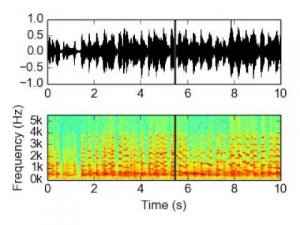
Figure 1: Spectrogram

Here, we can see that the spectrogram is representing portion of the graph where the signal is strong.

3. Fast Fourier Transform: FFT is used to compute Discrete Fourier Transform easily. DFT is used to transform configuration space to frequency space. According to fourier theorem, a signal is composition of a number of sinusoidal functions with given amplitude, frequency and phase. The fourier series equation formulates the theorem for periodic signal, x(t):

  X(t) = A0/2 + Σ (An sin(2πnt/p + φn) = Σ(Cne^(2πjnt/P)

 In these equations, P stands for the signals period and Cn is called Fourier coefficient of the signal x(t). The coefficients are calculated by:

Cn  = 1/p ∫ e ^ – (2Ï€jnt / p) x(t) dt

Now since we have gone through basic concepts required for starting with audio dataset, let us start with specific machine learning problem. The first of which will be speech classification.

4. Mel Frequency Ceptral Coefficient: MFCC is a feature taking process based on discrete fourier transforms. It is most generally used method for speech processing.  Cepstrum is the information of the rate of change in spectral bands, simply squared magnitude of the inverse Fourier transform of the logarithm of the squared magnitude of the Fourier transform of a signal.  In the conventional analysis of time signals, any periodic component shows up as sharp peaks in the corresponding frequency spectrum.

Mel Scale is a scale that relates perceived frequency of a tone to the actual measured frequency. It scales the frequency in order to match it closely to what humans can hear. It is represented by:

Mel(f) = 2595log(1 + f / 700)

5. Mel Frequency Warping:Mel Frequency Warping is commonly carried out by using filterbank which is one form of filter made with purpose to determine energy size of particular band in frequency. In context of MFCC filterbank should be applied to frequency domain. Filterbank uses convolution representation  to convert filter to signal. Convolution can be done by multiplication between signal spectrum with filter bank coefficient.

6. Windowing:Windowing is the process of filtering each frame by multiplying each frame with certain windows functions at the same time frame. Windowing is also used to ensure continuous sound from initial frame to end frame.

7.  Framing:Sound signals are not stationary signals, meaning their statistical properties are always changing in time. So it is not possible to extract the spectral features of speech at once. Therefore, the spectral character of sound signals is extracted through a window as a sound signal characterizing a particular sound part so that an assumption can be made that sound signals is stationary.

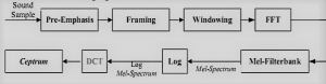
Figure 2: MFCC Process

Now, we have been familiar with some basic concepts required for starting with speech dataset we can start speech classification.

Firstly we have to load audio data using library like librosa.

X = []

y = []

pad = lambda a, i: a[0: i] if a.shape[0] > i else np.hstack((a, np.zeros(i – a.shape[0])))

for fname in os.listdir(DATA_DIR):

   struct = fname.split(‘_’)

   digit = struct[0]

   wav, sr = librosa.load(DATA_DIR + fname)

   padded = pad(wav, 30000)

   X.append(padded)

   y.append(digit)

X = np.vstack(X)

y = np.array(y)

Here, we are trying to classify spoken digit. In line wav, sr = librosa.load(“____”), wav is audio wave file in array format and sr is sampling rate.

We will use a simple MLP network with single hidden layer for start:

ip = Input(shape=(X[0].shape))

hidden = Dense(128, activation=’relu’)(ip)

op = Dense(10, activation=’softmax’)(hidden)

model = Model(input=ip, output=op)

model.summary()

Now let us train it.

model.compile(loss=’categorical_crossentropy’,

             optimizer=’adam’,

             metrics=[‘accuracy’])

history = model.fit(train_X,

         train_y,

         epochs=10,

         batch_size=32,

         validation_data=(test_X, test_y))

plt.plot(history.history[‘acc’], label=’Train Accuracy’)

plt.plot(history.history[‘val_acc’], label=’Validation Accuracy’)

plt.xlabel(‘Epochs’)

plt.ylabel(‘Accuracy’)

plt.legend()

With this method we get very less accuracy value. So, we introduce extra preprocessing in input dataset before they are fed in machine learning models like FFT.

fft = np.fft.fft(signal)[:50]

fft = np.abs(fft)

plt.plot(fft)

Now we also have to break recordings into small window and compute what frequency is there in each window so capture information from continuously changing audio file. We will use short fourier transform for this.

D = librosa.amplitude_to_db(np.abs(librosa.stft(wav)), ref=np.max)

librosa.display.specshow(D, y_axis=’linear’)

Here, librosa.stft computes short fourier transform and librosa.amplitude_to_db converts values to decibel.

Now, we are able to compute spectrograms for each file in our dataset and use them to classify digits. Spectrogram are in 2D format so we can pass them through convolutional neural network.

ip = Input(shape=train_X_ex[0].shape)

m = Conv2D(32, kernel_size=(4, 4), activation=’relu’, padding=’same’)(ip)

m = MaxPooling2D(pool_size=(4, 4))(m)

m = Dropout(0.2)(m)

m = Conv2D(64, kernel_size=(4, 4), activation=’relu’)(ip)

m = MaxPooling2D(pool_size=(4, 4))(m)

m = Dropout(0.2)(m)

m = Flatten()(m)

m = Dense(32, activation=’relu’)(m)

op = Dense(10, activation=’softmax’)(m)

model = Model(input=ip, output=op)

model.summary()

Now, the performance is a little better. For better result one can consult techniques of preprocessing like MFCC.

All of the above steps are explained in detail in this post:

https://towardsdatascience.com/speech-classification-using-neural-networks-the-basics-e5b08d6928b7

Now, we will go through other applications of machine learning with speech dataset which is Speaker Verification. It is one of the applications of speaker recognition technique. In this a speaker identity is verified. Whereas other application is identity verification in which an unknown speaker identity is to be determined.

It can be further classified in two:

1. Text – Dependent: This is the speaker verification process in which a talker should provide exact words, passwords.
2. Text – Independent: In this method a talker is not required to provide exact phrases for verification.

There is an implementation in github for speaker verification which gives result with good accuracy. The link is:

https://github.com/Janghyun1230/Speaker_Verification
Here, we will discuss in brief how this implementation can be used and details of specific files in each implementation. You can download required dataset from http://homepages.inf.ed.ac.uk/jyamagis/page3/page58/page58.html and noise from https://datashare.is.ed.ac.uk/handle/10283/1942 .

We can choose between tdsv or tisv by setting tdsv true or false, path for train_data directory,  test_data directory, noise_directory can be passed to configuration.py. data_preprocess.py is to extract features from speech dataset.So, we have to pass audio_path, clean_path and noise_path according to our file path format. Then model.py has LSTM model which is used for speaker verification. Here, you can change file path of checkpoint if necessary.

Now, you can begin training by passing,

python main.py –train True –model_path where_you_want_to_save

And can apply testing by,

python main.py –train False –model_path model_path used at training phase

After few epochs you will get output in format,

inference time for 40 utterances : 1.64s

[[[ 0.73 -0.43 -0.3 0. ]

[ 0.65 -0.42 -0.47 -0.39]

[ 0.62 -0.42 -0.48 -0.4 ]

[ 0.96 -0.28 -0.14 -0.05]

[ 0.68 -0.54 -0.4 -0.08]]

[[ 0.11 0.83 0.37 -0.24]

[-0.08 0.86 0.49 -0.24]

[-0.08 0.87 0.48 -0.25]

[-0.15 0.96 0.69 0.08]

[-0.17 0.97 0.68 0.01]]

[[-0.04 0.65 0.89 -0.05]

[-0.02 0.7 0.94 -0.01]

[-0.03 0.69 0.94 -0.04]

[-0.14 0.79 0.96 0.08]

[-0.07 0.75 0.89 0.06]]

[[-0.16 -0.13 0.07 0.88]

[-0.05 -0.18 0.1 0.95]

[-0.05 -0.24 0.08 0.94]

[-0.05 -0.09 0.31 0.93]

[-0.06 -0.18 0.06 0.91]]]

EER : 0.10 (thres:0.65, FAR:0.10, FRR:0.10)

This is the result of four speaker with five utterances. If you train it for more time you can verify decrease in ERR which is equal to false acceptance ratio, false rejection ratio. The result can also be viewed in tensorboard. The above result is similarity matrix which can be understood with given figure.

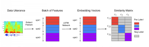
Figure 3: Similarity Matrix

Now, we will go through other task in machine learning on speech dataset which is text transcription. It means converting speech to text. For this you can use google API. But it converts audio about thirty seconds only. Here is a simple code that takes audio input from user and recognizes it.

import speech_recognition as sr

r = sr.Recognizer()

with sr.Microphone() as source:

   print(“Say Anything”)

   audio = r.listen(source)

try:

   text = r.recognize_google(audio).encode(‘utf-8’)

   print(“Here is what you said”, text)

except:

   print(“Translation Failed.”)

Similarly, here is a program to take input from audio file and transcribe it.

import speech_recognition as sr

from os import path

from pprint import pprint

import unicodedata

audio_file = path.join(path.dirname(path.realpath(__file__)), “data/A_very_good_news_for_Nepal-7hmCKv71PeM.wav”)

r = sr.Recognizer()

with sr.AudioFile(audio_file) as source:

audio = r.record(source)

try:

text = r.recognize_google(audio, show_all= True, language= ‘ne-NP’)

# text = unicodedata.normalize(‘NFKD’, text).encode(‘ISO-8859-1’, ‘ignore’)

print(text[u’alternative’][0][u’transcript’])

except:

   print(“IT did not work”)

Here, you can pass any language that is supported by google. I have passed ne-NP. Thus, it recognizes nepali speech.

The other problem that can be explored as application of machine learning to speech dataset is speaker diarization. It is one of the most complex problems in machine learning. It is about who spoke when. This task is sometimes confused with speaker recognition but speaker diarization is about recognizing when the same speaker is speaking whereas speaker recognition is about identifying who is speaking. It is also sometimes confused with speaker change detection. But they are also different as diarization labels when new speaker appears again whereas in speaker change detection no such labels are given.

According to the article on google speaker diarization is the process of partitioning an audio stream with multiple people into homogeneous segments associated with each individual and is an important part of speech recognition systems. By solving the problem of “who spoke when”, speaker diarization has applications in many important scenarios, such as understanding medical conversations, video captioning, call center data analysis, broadcast news, automatic note generation for meetings and many more.

There are many difficulties in the task of speaker diarization.

1. There might me multiple speaker speaking at the same time.
2. Data might contain music or non human utterances.
3. Audio recording condition might be different.
4. Number of speakers is not known in advance.
5. Identity of people is not known in advance.

 

Internal Working and Infrastructure of Diarization:

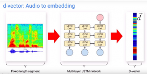
Figure 5: D- vector Embedding

1. Speech Detection: Voice activity detector is used to remove noise and non speech.
2. Speech Segmentation: Extract short segments from audio and run LSTM to produce D vector for each sliding window.
3. Embedding Extraction: For each segment aggregate the D vector belong to that segment to produce segment wise embeddings.
4. Clustering: Finally cluster the segment wise embedding to produce diarization result. Determine the number of speakers with each speaker timestamp.

The infrastructure of diarization after VAD can be visualized as:

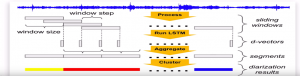
Figure 6: VAD Process

We can use spectral clustering to separate different speakers. Spectral makes a use of eigen value and affinity matrix to find clusters which is explained in this video:

https://www.youtube.com/watch?v=P-LEH-AFovE
Google has recently open sourced its speaker diarization implementation. It is available here https://github.com/google/uis-rnn.